
As we explored in previous sections on classification and feature selection, gene expression data can reliably identify cancer subtypes. Next, we will investigate whether it is possible to uncover subtype separations in an unsupervised manner using only transcriptomic data. Specifically, we will employ clustering techniques to group samples based on their similarities.
1. Hierarchical Clustering
The definition of similarity, especially between clusters, can significantly impact the outcomes of hierarchical clustering. Generally, clustering methods calculate the similarities between individual samples and then aggregate these similarities into a collective measure for the clusters. Each method utilizes a specific metric for similarity computation.
In this study, I applied agglomerative (bottom-up) hierarchical clustering, which begins by assigning each sample to its own distinct cluster. The algorithm identifies the pair of most similar samples and merges them into a single cluster, treating them as a “quasi-sample.” This merging process continues until all samples are consolidated into one cluster. The results are typically visualized as a dendrogram, which illustrates the sequence in which clusters are merged. The height of the branches in this tree indicates the level of similarity between clusters; greater heights reflect higher dissimilarity. By cutting the dendrogram at a specific height, I can achieve clusters of desired sizes—making a cut closer to the leaves results in more smaller clusters, while a cut near the root yields fewer larger clusters.
1.1. Input
For this analysis, I utilized a dataset comprising 52 samples of 7,000 genes as input for clustering.
| ID | S01 | S02 | S03 | S04 | S05 | S06 | S07 | S08 | S09 | S10 | S11 | S12 | S13 | S14 | S15 | S16 | S17 | S18 | S19 | S20 | S21 | S22 | S23 | S24 | S25 | S26 | S27 | S28 | S29 | S30 | S31 | S32 | S33 | S34 | S35 | S36 | S37 | S38 | S39 | S40 | S41 | S42 | S43 | S44 | S45 | S46 | S47 | S48 | S49 | S50 | S51 | S52 |
|---|---|---|---|---|---|---|---|---|---|---|---|---|---|---|---|---|---|---|---|---|---|---|---|---|---|---|---|---|---|---|---|---|---|---|---|---|---|---|---|---|---|---|---|---|---|---|---|---|---|---|---|---|
| ENSG00000000419 | 6.038 | 5.219 | 5.115 | 5.326 | 5.186 | 5.287 | 5.268 | 6.624 | 5.571 | 6.597 | 5.211 | 6.652 | 6.611 | 6.395 | 5.151 | 6.138 | 7.278 | 4.737 | 6.125 | 5.63 | 5.777 | 6.18 | 4.644 | 6.481 | 5.724 | 5.459 | 4.74 | 7.281 | 5.198 | 5.609 | 4.776 | 5.615 | 6.047 | 4.743 | 6.229 | 5.152 | 5.778 | 4.583 | 5.963 | 6.168 | 4.925 | 4.074 | 5.797 | 6.381 | 4.624 | 5.986 | 6.375 | 7.702 | 5.679 | 5.832 | 5.308 | 5.036 |
| ENSG00000001036 | 4.408 | 5.363 | 5.249 | 5.796 | 5.731 | 6.092 | 4.759 | 4.412 | 4.953 | 6.929 | 4.959 | 5.074 | 5.39 | 4.528 | 4.696 | 6.009 | 5.443 | 4.256 | 6.142 | 5.864 | 5.341 | 5.992 | 4.676 | 5.139 | 6.946 | 5.942 | 6.075 | 6.336 | 4.982 | 5.277 | 6.352 | 5.205 | 6.271 | 5.783 | 4.085 | 6.551 | 5.889 | 5.155 | 3.923 | 5.453 | 4.065 | 5.878 | 5.485 | 5.107 | 6.206 | 5.034 | 5.27 | 5.734 | 5.365 | 4.205 | 4.986 | 5.652 |
| ENSG00000001084 | 4.417 | 5.983 | 5.749 | 5.736 | 5.738 | 5.758 | 3.925 | 5.101 | 5.073 | 3.528 | 5.907 | 4.03 | 3.577 | 3.093 | 4.969 | 5.789 | 4.443 | 5.138 | 5.585 | 6.172 | 4.977 | 6.776 | 5.952 | 4.72 | 4.586 | 5.829 | 3.988 | 4.735 | 4.201 | 6.793 | 6.236 | 4.439 | 5.045 | 5.176 | 4.172 | 4.044 | 5.978 | 4.084 | 3.042 | 4.221 | 3.871 | 5.231 | 6.616 | 4.314 | 6.365 | 4.468 | 4.084 | 3.095 | 4.29 | 2.249 | 5.871 | 4.303 |
| ENSG00000001497 | 5.242 | 4.2 | 6.563 | 5.509 | 5.539 | 4.889 | 6.14 | 5.325 | 5.067 | 6.147 | 5.469 | 6.077 | 6.871 | 5.967 | 6.682 | 4.986 | 5.3 | 6.449 | 4.947 | 5.46 | 5.438 | 5.933 | 3.964 | 4.578 | 6.386 | 4.93 | 4.866 | 6.102 | 4.718 | 5.275 | 4.747 | 5.592 | 5.071 | 5.305 | 4.131 | 5.444 | 3.832 | 5.106 | 5.93 | 4.696 | 4.91 | 5.225 | 4.644 | 6.144 | 5.069 | 4.746 | 4.907 | 5.808 | 4.85 | 5.3 | 4.157 | 6.014 |
| ENSG00000001617 | 6.028 | 7.304 | 3.906 | 5.913 | 5.957 | 3.985 | 7.524 | 4.648 | 6.675 | 3.168 | 5.361 | 6.536 | 6.393 | 5.222 | 1.325 | 3.853 | 4.694 | 4.617 | 2.5 | 3.199 | 5 | 5.301 | 5.471 | 5.007 | 1.436 | 5.811 | 2.974 | 3.771 | 7.3 | 5.09 | 5.116 | 5.192 | 5.487 | 6.753 | 5.083 | 0.373 | 5.46 | 7.737 | 0.795 | 6.797 | 1.26 | 4.758 | 3.704 | 5.568 | 5.234 | 4.296 | 5.062 | 6.554 | 6.172 | 6.783 | 4.914 | 5.93 |
| … | … | … | … | … | … | … | … | … | … | … | … | … | … | … | … | … | … | … | … | … | … | … | … | … | … | … | … | … | … | … | … | … | … | … | … | … | … | … | … | … | … | … | … | … | … | … | … | … | … | … | … | … |
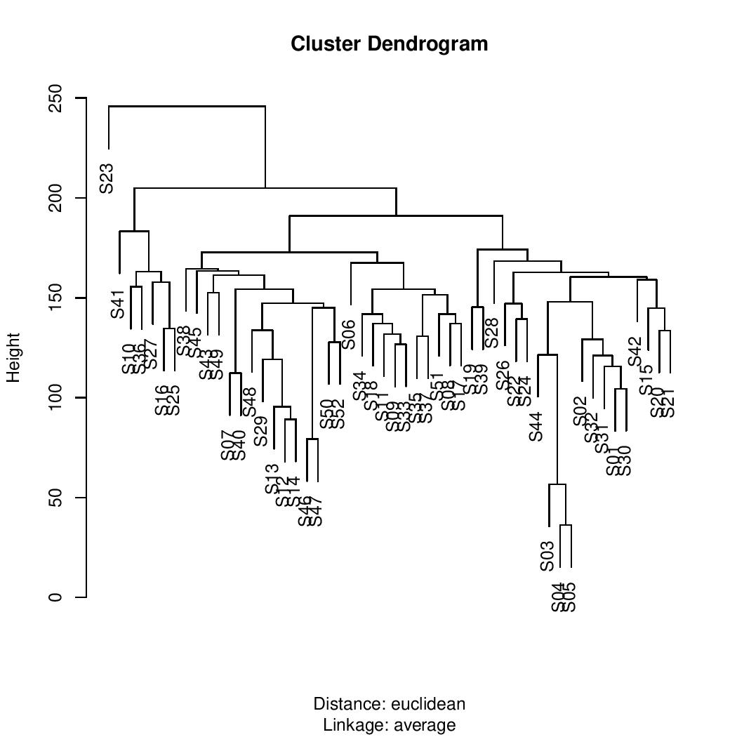
1.2. Result
The resulting dendrogram revealed that similar samples were grouped together. For instance, samples S03, S04, and S05 formed a small branch, while S12, S13, and S14 were located in a branch significantly distant from the first.
If the number of clusters is set to five, the algorithm will return the assigned cluster for each sample.
| Sample | Cluster ID |
|---|---|
| S01 | 1 |
| S02 | 1 |
| S03 | 1 |
| S04 | 1 |
| S05 | 1 |
| S06 | 2 |
| S07 | 2 |
| S08 | 2 |
| S09 | 2 |
| S10 | 3 |
| S11 | 2 |
| S12 | 2 |
| S13 | 2 |
| S14 | 2 |
| S15 | 1 |
| S16 | 3 |
| S17 | 2 |
| S18 | 2 |
| S19 | 1 |
| S20 | 1 |
| S21 | 1 |
| S22 | 1 |
| S23 | 4 |
| S24 | 1 |
| S25 | 3 |
| S26 | 1 |
| S27 | 3 |
| S28 | 1 |
| S29 | 2 |
| S30 | 1 |
| S31 | 1 |
| S32 | 1 |
| S33 | 2 |
| S34 | 2 |
| S35 | 2 |
| S36 | 3 |
| S37 | 2 |
| S38 | 2 |
| S39 | 1 |
| S40 | 2 |
| S41 | 3 |
| S42 | 1 |
| S43 | 2 |
| S44 | 1 |
| S45 | 2 |
| S46 | 2 |
| S47 | 2 |
| S48 | 2 |
| S49 | 2 |
| S50 | 2 |
| S51 | 2 |
| S52 | 2 |
2. K-means Clustering
Another commonly used clustering method is k-means. In k-means, the number of clusters, “K,” is set as an input parameter at the beginning, and “K” initial centroids are randomly selected within the sample space. Each sample is then assigned to the cluster associated with the nearest centroid. After the initial assignments, the algorithm updates each cluster’s centroid to reflect the actual mean of the samples it contains, and the process iterates with these new centroids. This cycle continues until convergence is reached or a predefined stopping condition is met, such as the maximum number of iterations.
It is important to note that due to random initialization, running k-means multiple times with the same parameters on the same data can yield different results, especially if the true clustering structure is not clear.
2.1. Input
We continue to work with the same input data of 52 samples as described in 1.1.
2.2. Result
The resulting table is straightforward, with each sample assigned to a cluster.
| Sample | Cluster ID |
|---|---|
| S01 | 1 |
| S02 | 1 |
| S03 | 1 |
| S04 | 1 |
| S05 | 1 |
| S06 | 3 |
| S07 | 2 |
| S08 | 3 |
| S09 | 3 |
| S10 | 4 |
| S11 | 3 |
| S12 | 2 |
| S13 | 2 |
| S14 | 2 |
| S15 | 1 |
| S16 | 4 |
| S17 | 3 |
| S18 | 3 |
| S19 | 1 |
| S20 | 1 |
| S21 | 1 |
| S22 | 1 |
| S23 | 3 |
| S24 | 1 |
| S25 | 4 |
| S26 | 1 |
| S27 | 4 |
| S28 | 1 |
| S29 | 2 |
| S30 | 1 |
| S31 | 1 |
| S32 | 1 |
| S33 | 3 |
| S34 | 3 |
| S35 | 3 |
| S36 | 4 |
| S37 | 3 |
| S38 | 2 |
| S39 | 1 |
| S40 | 2 |
| S41 | 4 |
| S42 | 1 |
| S43 | 2 |
| S44 | 1 |
| S45 | 2 |
| S46 | 2 |
| S47 | 2 |
| S48 | 2 |
| S49 | 2 |
| S50 | 2 |
| S51 | 3 |
| S52 | 3 |
It is advisable to repeat multiple runs to assess the accuracy that this method can provide on a particular dataset. If the results vary significantly across runs, it should be combined with prior knowledge or other methods to validate the findings.
Acknowledgement
These projects were supported by Louisiana Biomedical Research Network and Pine Biotech under LBRN Summer Bioinformatics Workshop in 2018.