
In my work with transcriptomics, I executed RNA-Seq pipelines, focusing on the importance of selecting the most appropriate algorithms for the data being analyzed. The project involved gene expression analysis using RNA-Seq data processed through RSEM for expression measurement. I further refined the data by filtering out genes with zero expression values and applying quantile normalization to ensure consistency across samples.
Once the data tables were prepared, I utilized machine learning algorithms to classify these subtypes automatically, identifying the most informative genes for distinguishing between the known classes.
1. Classification
Breast cancer was reported to be able divided into distinct subtypes. In this work, I worked on 38 datasets from 5 cell lines (luminal, basal, claudin-low, and normal-like cases). I wanted to identify the most informative features (genes) in these subtypes using supervised machine learning methods, specifically classification algorithms. In this case, I applied Linear Discriminant Analysis (LDA). LDA works similarly to Principal Component Analysis (PCA) but takes subtype information into account when determining the components. Like other classification methods, LDA uses a training set where the subtypes are already known. From this training set, LDA constructed a classifier that could then assign new samples to one of the known subtypes.
1.1. Input
The gene expression data and subtype information were combined into a single table to serve as the training set. Each sample (or cell line) was represented by a column and was labeled with its respective subtype. For this analysis, the subtypes were encoded as follows:
- B – Basal
- CL – Claudin-low
- L – Luminal
- N – Normal-like
| ID | S01 | S02 | S03 | S04 | S05 | S06 | S07 | S08 | S09 | S10 | S11 | S12 | S13 | S14 | S15 | S16 | S17 | S18 | S19 | S20 | S21 | S22 | S23 | S24 | S25 | S26 | S27 | S28 | S29 | S30 | S31 | S32 | S33 | S34 | S35 | S36 | S37 | S38 |
|---|---|---|---|---|---|---|---|---|---|---|---|---|---|---|---|---|---|---|---|---|---|---|---|---|---|---|---|---|---|---|---|---|---|---|---|---|---|---|
| class | Type_L | Type_L | Type_L | Type_L | Type_CL | Type_L | Type_L | Type_L | Type_L | Type_B | Type_CL | Type_L | Type_L | Type_B | Type_B | Type_B | Type_B | Type_L | Type_B | Type_B | Type_B | Type_L | Type_N | Type_N | Type_N | Type_L | Type_L | Type_L | Type_CL | Type_L | Type_L | Type_B | Type_L | Type_CL | Type_B | Type_L | Type_B | Type_L |
| ENSG00000000419 | 5.32 | 5.3 | 6.64 | 5.6 | 6.61 | 5.24 | 6.66 | 6.62 | 6.41 | 5.19 | 6.16 | 7.29 | 4.78 | 6.14 | 5.66 | 5.8 | 6.2 | 4.69 | 6.5 | 5.49 | 7.29 | 5.23 | 5.63 | 4.82 | 5.64 | 6.07 | 4.79 | 6.25 | 5.19 | 5.8 | 4.63 | 5.98 | 6.19 | 4.97 | 4.15 | 5.82 | 6.4 | 4.67 |
| ENSG00000001036 | 6.11 | 4.8 | 4.47 | 4.99 | 6.94 | 5 | 5.11 | 5.42 | 4.58 | 4.74 | 6.03 | 5.47 | 4.32 | 6.16 | 5.89 | 5.37 | 6.01 | 4.72 | 5.17 | 5.96 | 6.35 | 5.02 | 5.31 | 6.37 | 5.24 | 6.29 | 5.81 | 4.16 | 6.56 | 5.91 | 5.19 | 4 | 5.48 | 4.14 | 5.9 | 5.51 | 5.14 | 6.22 |
| ENSG00000001084 | 5.78 | 4.01 | 5.14 | 5.11 | 3.63 | 5.93 | 4.11 | 3.68 | 3.23 | 5.01 | 5.81 | 4.5 | 5.17 | 5.61 | 6.19 | 5.02 | 6.79 | 5.97 | 4.77 | 5.85 | 4.78 | 4.27 | 6.8 | 6.25 | 4.5 | 5.08 | 5.21 | 4.24 | 4.12 | 6 | 4.16 | 3.19 | 4.29 | 3.95 | 5.26 | 6.63 | 4.38 | 6.38 |
| … | … | … | … | … | … | … | … | … | … | … | … | … | … | … | … | … | … | … | … | … | … | … | … | … | … | … | … | … | … | … | … | … | … | … | … | … | … | … |
For the test set, I used a similar table that did not include class labels, allowing LDA to predict the subtypes.
| ID | T01 | T02 | T03 | T04 | T05 | T06 | T07 | T08 | T09 | T10 | T11 | T12 | T13 | T14 |
|---|---|---|---|---|---|---|---|---|---|---|---|---|---|---|
| ENSG00000000419 | 6.06 | 5.25 | 5.15 | 5.36 | 5.22 | 5.75 | 4.79 | 6.01 | 6.39 | 7.71 | 5.7 | 5.85 | 5.34 | 5.07 |
| ENSG00000001036 | 4.47 | 5.39 | 5.28 | 5.82 | 5.75 | 6.96 | 6.09 | 5.07 | 5.3 | 5.76 | 5.4 | 4.27 | 5.03 | 5.68 |
| ENSG00000001084 | 4.47 | 6 | 5.77 | 5.76 | 5.76 | 4.64 | 4.07 | 4.52 | 4.16 | 3.24 | 4.35 | 2.49 | 5.89 | 4.37 |
| ENSG00000001497 | 5.27 | 4.27 | 6.58 | 5.54 | 5.57 | 6.4 | 4.91 | 4.79 | 4.95 | 5.83 | 4.89 | 5.33 | 4.23 | 6.03 |
| … | … | … | … | … | … | … | … | … | … | … | … | … | … | … |
1.2. Result
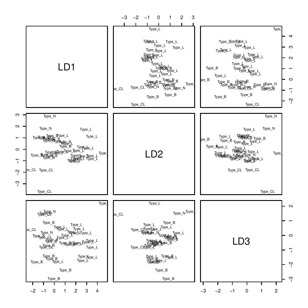
The effectiveness of the LDA classifier constructed for the training set could be assessed by examining the results presented in LDA_plot. For example, the first two axes achieved a separation of type N (Normal-like) and type CL (Claudin-low).
LDA plot
Another results provided by LDA was the confusion matrix, which presents the predicted classifications in rows against the actual classifications in columns. The diagonal elements represented the number of correct predictions (true positives), while the values above the diagonal indicate true observations that were not predicted (false negatives), and those below represent predictions that were incorrect (false positives). According to this matrix, the classification accuracy for the training set was around 87%.
Prediction result
| Sample | Class |
|---|---|
| T01 | Type_B |
| T02 | Type_B |
| T03 | Type_B |
| T04 | Type_B |
| T05 | Type_B |
| T06 | Type_CL |
| T07 | Type_B |
| T08 | Type_L |
| T09 | Type_L |
| T10 | Type_L |
| T11 | Type_L |
| T12 | Type_L |
| T13 | Type_L |
| T14 | Type_L |
Confusion matrix
| True predicted | Type_B | Type_CL | Type_L | Type_N |
|---|---|---|---|---|
| Type_B | 9 | 1 | 1 | 1 |
| Type_CL | 0 | 3 | 0 | 0 |
| Type_L | 1 | 0 | 19 | 0 |
| Type_N | 1 | 0 | 0 | 2 |
In addition to LDA, various classification methods, including Support Vector Machine (SVM), Random Forest, and Naive Bayes were introduced. Each of these methods employs different mathematical approaches to tackle the same classification task, providing multiple options for the best fit for specific data and analysis purposes.
2. Feature Selection
One effective method for this was stepwise feature selection. Similar to LDA, this approach begins by testing individual features and selecting the one that provides the best classification quality for the training set. The process then evaluates pairs of features, where the first feature is the previously selected one, and identifies the pair that yields the highest classification accuracy. This method continues with triples, quadruples, and so forth. Although this greedy strategy may not be optimal, it delivers results within a reasonable timeframe.
2.1. Input
To implement this, I utilized the swLDA (step-wise LDA) algorithm, using the same training and testing datasets.
2.2. Result
Unlike LDA, swLDA required an additional parameter called Niveau, which determines the stopping criterion. This parameter should be adjusted based on the size of the transcriptome; in this case, with nearly 7,000 genes, I set it to 0.0005.
Prediction result
| Sample | Class |
|---|---|
| T01 | Type_N |
| T02 | Type_B |
| T03 | Type_B |
| T04 | Type_B |
| T05 | Type_B |
| T06 | Type_CL |
| T07 | Type_CL |
| T08 | Type_L |
| T09 | Type_L |
| T10 | Type_L |
| T11 | Type_L |
| T12 | Type_L |
| T13 | Type_L |
| T14 | Type_L |
Confusion matrix
| True predicted | Type_B | Type_CL | Type_L | Type_N |
|---|---|---|---|---|
| Type_B | 11 | 0 | 0 | 0 |
| Type_CL | 0 | 4 | 0 | 0 |
| Type_L | 0 | 0 | 20 | 0 |
| Type_N | 0 | 0 | 0 | 3 |
swLDA plot
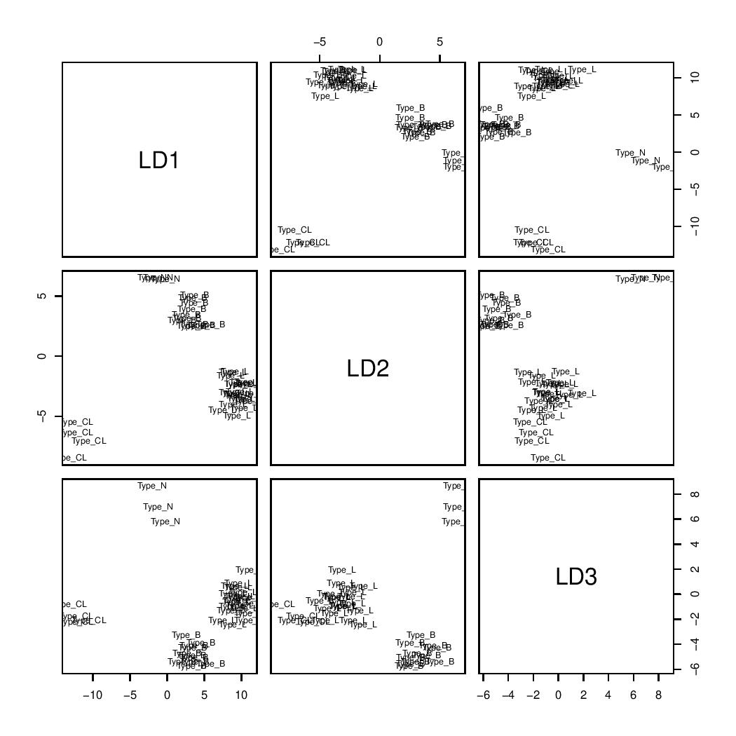
Compared to LDA, swLDA achieved a higher accuracy in subtype classification, with a prediction rate of 100%. The feature mean and coefficient tables below revealed that 7 genes were selected, which enabled perfect classification of the training set.
swLDA_Features_means
| Class | ENSG00000116299 | ENSG00000166145 | ENSG00000243509 | ENSG00000119888 | ENSG00000168918 | ENSG00000261040 | ENSG00000049283 |
|---|---|---|---|---|---|---|---|
| Basal | 1.1 | 7.2 | 0.4 | 6.9 | 0.1 | 2.0 | 4.7 |
| Claudin-low | 0.7 | 0.8 | 1.4 | 0.7 | 0.2 | 3.9 | 0.2 |
| Luminal | 6.5 | 7.7 | 0.4 | 7.0 | 1.1 | 0.5 | 6.5 |
| Normal-like | 0.5 | 6.6 | 5.8 | 3.9 | 3.4 | 4.2 | 1.1 |
swLDA_Features_coeffs
| scaling LD1 | scaling LD2 | scaling LD3 | |
|---|---|---|---|
| ENSG00000116299 | 0.8 | -1.1 | 0.5 |
| ENSG00000166145 | 1.0 | 1.0 | 0.1 |
| ENSG00000243509 | 0.0 | 0.4 | 1.6 |
| ENSG00000119888 | 1.0 | 1.3 | -0.3 |
| ENSG00000168918 | 0.4 | 0.6 | 1.0 |
| ENSG00000261040 | -0.3 | 0.3 | -0.8 |
| ENSG00000049283 | 0.5 | -0.6 | -0.4 |
Acknowledgement
These projects were supported by Louisiana Biomedical Research Network and Pine Biotech under LBRN Summer Bioinformatics Workshop in 2018.